Discretization#

NeuralMag offers two closely related spatial discretizations on a regular cuboid grid. Both share the same form compiler and the same FFT demagnetization kernel; they differ only in where the magnetization lives:

Scheme	`m` lives on	Field `h` is computed on
Nodal FD	nodes (trilinear basis)	nodes
FIC (cell-centred)	cells (piecewise constant)	nodes, projected back to cells

Pick whichever is more natural for the problem at hand — see the Choosing a scheme section below — and then forget about the difference: the rest of the API is identical.

The mesh and notation#

A Mesh is a regular cuboid grid characterised by

the number of cells in each principal direction, n = (n_x, n_y, n_z);
the cell size, dx = (dx_x, dx_y, dx_z);
an optional origin.

Throughout this page we use \(i, j, k\) for cell indices (running from 0 to n_*-1) and \(I, J, K\) for node indices (running from 0 to n_*). Material parameters such as \(A_\text{ex}\) or \(M_\text{s}\) are always piecewise-constant on cells.

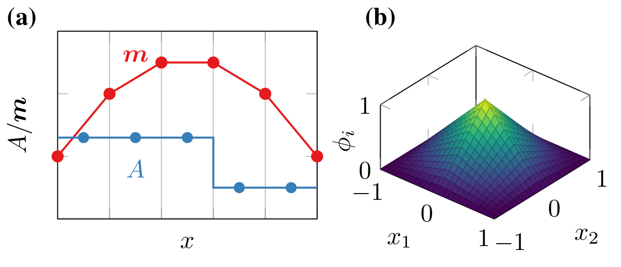
../_images/nodal_fd.png — Fig. 1 Regular cuboid grid in NeuralMag. (a) 1D representation of the discretization for a continuous field (red) and piecewise-constant material parameters (blue). (b) 2D trilinear basis function \(\phi_i(x_1, x_2)\).#

Nodal finite-difference scheme (default)#

The default scheme is the nodal finite-difference method introduced for NeuralMag by Abert et al. (npj Comput. Mater. 11, 193, 2025). Despite the name it is, strictly speaking, a finite-element method on a structured grid with the standard FD savings: because the mesh is regular, every element matrix is identical and we never have to assemble or store a global matrix.

Function spaces#

The magnetization \(\vec m\) lives in a continuous, piecewise trilinear Lagrange space attached to the mesh nodes (basis functions \(\phi_{IJK}\)).
Material parameters such as \(M_\text{s}\), \(A_\text{ex}\), \(K_\text{u}\) live in a piecewise-constant space attached to the cells (basis functions \(\theta_{ijk}\)).

This is exactly the standard mixed setup that lets sharp material interfaces land on cell boundaries while keeping the magnetization continuous across them — a small but essential property when you compare numerics against analytical interface models.

Effective field via mass lumping#

The discrete effective field at node \(i\) is obtained from the energy functional \(E[\vec m]\) via a mass-lumped weak form:

\[H_i \;=\; -\,\Bigl[\,\int_{\Omega_\text{m}} \mu_0 M_\text{s}\, \vec\phi_i\cdot\vec 1\,\dx\Bigr]^{-1}\, \frac{\delta E}{\delta \vec m}\bigl|_{\vec\phi_i},\]

where the term in square brackets is the diagonal lumped mass at node \(i\) and \(\delta E/\delta\vec m\bigl|_{\vec\phi_i}\) is the Gâteaux derivative of \(E\) in the direction of the basis function \(\vec\phi_i\). For a quadratic energy (e.g. exchange), this becomes a constant linear operator

\[H_i \;=\; \sum_j A_{ij}\, m_j, \qquad A_{ij} \;=\; - \Bigl[\!\int_{\Omega_\text{m}} \mu_0 M_\text{s}\,\vec\phi_i\cdot\vec 1\,\dx\Bigr]^{-1}\! \int_{\Omega_\text{m}} A_\text{ex}\, \nabla\vec\phi_i : \nabla\vec\phi_j \dx.\]

Because the grid is regular, \(A_{ij}\) has a translation-invariant stencil structure and is never assembled: NeuralMag’s form compiler emits a few vectorized array slices that compute \(H_i\) directly from the m tensor (see Form Compiler). This is what gives the scheme its finite-difference price tag.

Demag#

For the demagnetization field NeuralMag uses the FFT-accelerated convolution of magnum.np, the same well benchmarked kernel as in classical FD codes. Combining the speed of FFT demag with the interface accuracy of the nodal finite-difference scheme is the central practical reason to prefer NeuralMag over a pure FD code.

When to prefer the nodal scheme

Smooth magnetization fields and well-resolved domain walls.
Standard micromagnetic benchmark problems (Standard Problem 4, etc.).
Anything that you would solve with a finite-element micromagnetic code today and where you want a familiar mental model.

FIC — cell-centred variant#

FIC stores the magnetization at cell centres but computes the effective field with the same nodal finite-difference machinery as above. The bridge between the two layouts is a pair of mass-lumped \(L^2\) projections that the form compiler generates from very short symbolic expressions.

Conceptually, every effective-field evaluation runs three steps:

Cell → node projection of m: solve

\[\int_{\Omega_\text{m}} \vec v_n\cdot\vec m_c \dx \;=\; \langle \vec v_n,\vec m_n\rangle_{\text{lumped}}\]

for the nodal coefficients \(\vec m_n\), with mass lumping (single-point quadrature, n_gauss = 1) so the system is diagonal.
Standard nodal finite-difference computation of the field \(\vec H_n\) from \(\vec m_n\), exactly as in Nodal finite-difference scheme (default).
Node → cell projection of the resulting field, using the dual mass-lumped form

\[\int_{\Omega_\text{m}} \vec v_c\cdot\vec H_n \dx \;=\; \langle \vec v_c,\vec H_c\rangle_{\text{lumped}}.\]

The energy density is projected the same way (a scalar \(\int v_c\, e_n\,\dx\) form). All three projection forms are written as plain SymPy expressions and emitted through the same code generator the rest of NeuralMag uses; you can read the exact code in neuralmag/field_terms/field_term.py (the _generate_kernel_code classmethod, where m is projected to nodes, the field is assembled, and the result is projected back to state.m.spaces).

In a FIC simulation you only see the cell-centred view: state.m is a VectorCellFunction, state.h_demag returns a tensor of shape (n_x, n_y, n_z, 3), and so on. The node-side intermediates exist only inside the generated function.

When to prefer FIC

Topology optimization, where the design variable \(\rho\) and the material parameters live naturally on cells.
Geometries imported from imaging or CAD pipelines that produce cell-aligned masks.
Interfaces that should remain sharp in the discretization rather than being smeared by trilinear interpolation of m.

Choosing a scheme#

A short rule of thumb:

Situation	Use
Standard problems / smooth fields	nodal FD
Topology optimization (cell-based design vars)	FIC
Sharp material interfaces, voxel data	FIC
Comparing against existing FE micromagnetic codes	nodal FD

If you switch later you only need to change state.m from a VectorFunction to a VectorCellFunction (or vice versa) — every field term re-detects the layout from state.m.spaces and re-compiles its code on the next access.