Composite chiral magnet benchmark#
This example reproduces the benchmark problem introduced in
Laliena, S. A. Osorio, S. Bustingorry, and J. Campo. Continuum of metastable helical states of monoaxial chiral magnets: Effect of boundary conditions. Physical Review B, 109:214424, 2024.
A one-dimensional composite consisting of a chiral slab sandwiched between two ferromagnetic slabs is relaxed to its ground state. Because the Dzyaloshinskii–Moriya interaction (DMI) is non-zero only inside the chiral region, the ground state is a Bloch helix in the centre that is matched to exponentially decaying profiles in the outer ferromagnetic regions. Laliena et al. provide a closed-form analytical solution that we use to validate the numerical simulation.
Problem setup#
The system is symmetric about \(x=0\) and occupies \(|x|\le L=150\,\mathrm{nm}\). The chiral region covers \(|x|\le L_0=100\,\mathrm{nm}\) and uses exchange \(A\), bulk DMI constant \(D\) and easy-plane anisotropy \(K_c = -(h_c-1)\,D^2/A\) with reduced field \(h_c=6\). The ferromagnetic slabs use exchange \(\rho\,A\) (with \(\rho=3\)), \(D=0\) and easy-axis anisotropy \(K_u = \rho\,D^2/(4A)\) with easy axis along \(\hat{\mathbf y}\).
The ground state is the Bloch helix \(\mathbf m = (0,\cos\varphi,\sin\varphi)\) where the phase \(\varphi\) satisfies
with \(q_0 = D/(2A)\) and a pitch parameter \(p\) that is fixed by matching the flux \(2A\varphi' - D\) across the chiral–ferro interface at \(x=\pm L_0\). Outside the chiral region the phase obeys the pendulum equation \(\varphi'' = q_u^2\sin\varphi\cos\varphi\) with \(q_u = q_0\).
Simulation#
Import libraries#
We import NumPy, SciPy and NeuralMag and set the default precision to double to guarantee convergence.
[1]:
import matplotlib.pyplot as plt
import numpy as np
from scipy.integrate import solve_ivp
from scipy.optimize import brentq

import neuralmag as nm

nm.config.dtype = "float64"
2026-04-07 18:17:03 NeuralMag:INFO [NeuralMag] Version 0.9.3
2026-04-07 18:17:04 NeuralMag:INFO [NeuralMag] Backend set to 'jax'.
2026-04-07 18:17:04 NeuralMag:INFO [NeuralMag] Set default dtype to 'float64'.
Material parameters and geometry#
All material constants are taken from the Laliena benchmark. The saturation magnetisation is \(M_s = 10^6\,\mathrm{A/m}\), the exchange constant in the chiral region is \(A = 10^{-11}\,\mathrm{J/m}\), and the bulk DMI constant is \(D = 4\,\mathrm{mJ/m^2}\). The exchange ratio between ferro and chiral region is \(\rho=3\) and the reduced anisotropy field is \(h_c=6\). The total length is \(2L = 300\,\mathrm{nm}\) discretised with cell size \(\Delta x = 0.5\,\mathrm{nm}\) (\(N=600\) cells).
[2]:
# Physical parameters
A = 1e-11  # Exchange constant [J/m]
D = 4e-3  # Bulk DMI constant [J/m²]
rho = 3.0  # Exchange ratio ferro/chiral
hc = 6.0  # Reduced anisotropy field
Ms = 1e6  # Saturation magnetization [A/m]
q0 = D / (2 * A)
qu = q0
Kc = -(hc - 1) * D**2 / A  # Easy-plane anisotropy (chiral)
Ku = rho * D**2 / (4 * A)  # Easy-axis anisotropy (ferro)

# Geometry
L0 = 100e-9  # Half-width of chiral region [m]
L = 150e-9  # Half-width of total system [m]
dx = 0.5e-9  # Cell size [m]
N = round(2 * L / dx)
Analytical solution#
The matching condition at \(x=\pm L_0\) determines the pitch parameter \(p\) as the root of
that lies closest to unity. We bracket and refine it with Brent’s method. The phase in the ferromagnetic slabs is then obtained by integrating the pendulum equation with initial conditions \(\varphi(L_0)=p\,q_0\,L_0\) and \(\varphi'(L_0)=(p-1)\,q_0/\rho\).
[3]:
def f_trans(p):
    return p - 1 + (rho * qu / q0) * np.sin(p * q0 * L0)


p_min = max(1 - np.sqrt(hc), 1 - rho * qu / q0)
p_max = min(1 + np.sqrt(hc), 1 + rho * qu / q0)
p_scan = np.linspace(p_min + 1e-10, p_max - 1e-10, 10000)
f_scan = f_trans(p_scan)
p_roots = []
for i in range(len(f_scan) - 1):
    if f_scan[i] * f_scan[i + 1] < 0:
        p_roots.append(brentq(f_trans, p_scan[i], p_scan[i + 1]))
p_val = np.array(p_roots)[np.argmin(np.abs(np.array(p_roots) - 1))]
print(f"pitch parameter p = {p_val:.6f}")
pitch parameter p = 0.943421
[4]:
def analytical_profile(x, p):
    phi = np.zeros_like(x)
    # chiral region: linear phase
    mc = np.abs(x) <= L0
    phi[mc] = p * q0 * x[mc]
    # right ferro region: integrate pendulum equation
    mr = x > L0
    if np.any(mr):
        xr = np.clip(x[mr], L0, L)
        sol = solve_ivp(
            lambda t, y: [y[1], qu**2 * np.sin(y[0]) * np.cos(y[0])],
            [L0, L],
            [p * q0 * L0, (p - 1) * q0 / rho],
            t_eval=xr,
            rtol=1e-12,
            atol=1e-14,
        )
        phi[mr] = sol.y[0]
    # left ferro region: use symmetry
    ml = x < -L0
    if np.any(ml):
        xl = np.clip(-x[ml][::-1], L0, L)
        sol = solve_ivp(
            lambda t, y: [y[1], qu**2 * np.sin(y[0]) * np.cos(y[0])],
            [L0, L],
            [p * q0 * L0, (p - 1) * q0 / rho],
            t_eval=xl,
            rtol=1e-12,
            atol=1e-14,
        )
        phi[ml] = -sol.y[0][::-1]
    return phi
Create mesh and state#
We use a 1D nodal mesh with \(N=600\) cells centred at the origin. The NeuralMag State holds all field quantities that live on this mesh.
[ ]:
mesh = nm.Mesh((N,), (dx, dx, dx), origin=(-L, 0, 0))
state = nm.State(mesh)

# cell-centre and node coordinates along x (x_c as backend tensor so the
# conditions fed to state.add_domain are valid for both jax and torch)
x_c = state.coordinates()[0]
x_n = -L + np.arange(N + 1) * dx
Material domains#
The two regions (chiral and ferromagnetic) are introduced via domain labels, and the material parameters are assigned per domain using fill_by_domain. Domain 0 (the background) has zero material, domain 1 is the chiral slab and domain 2 is the ferromagnetic slab. The easy-axis direction of the anisotropy is \(\hat{\mathbf x}\) (easy-plane \(y\)-\(z\)) in the chiral region and \(\hat{\mathbf y}\) in the ferro region.
[6]:
state.add_domain(1, abs(x_c) <= L0)
state.add_domain(2, abs(x_c) > L0)

state.material.Ms = nm.CellFunction(state).fill_by_domain([0.0, Ms, Ms])
state.material.A = nm.CellFunction(state).fill_by_domain([0.0, A, rho * A])
state.material.Db = nm.CellFunction(state).fill_by_domain([0.0, D, 0.0])
state.material.Ku = nm.CellFunction(state).fill_by_domain([0.0, Kc, Ku])
state.material.Ku_axis = nm.VectorCellFunction(state).fill_by_domain([[0, 0, 0], [1, 0, 0], [0, 1, 0]])
state.material.alpha = 1.0
Initial magnetisation#
We seed the simulation with the analytical helix profile. The phase is evaluated at cell centres, the resulting magnetisation is averaged onto the nodal mesh and renormalised. Starting from the analytical profile ensures that the LLG relaxation converges to the correct winding number.
[7]:
phi_n = analytical_profile(x_n, p_val)
m_init = np.zeros((N + 1, 3))
m_init[:, 1] = np.cos(phi_n)
m_init[:, 2] = np.sin(phi_n)

state.m = nm.VectorFunction(state, tensor=state.tensor(m_init))
Effective field and relaxation#
The total effective field contains contributions from exchange, bulk DMI and uniaxial anisotropy. After registering each contribution with the state, we relax the system to an energetic minimum with the Landau–Lifshitz–Gilbert solver.
[8]:
nm.ExchangeField().register(state, "exchange")
nm.BulkDMIField().register(state, "dmi")
nm.UniaxialAnisotropyField().register(state, "aniso")
nm.TotalField("exchange", "dmi", "aniso").register(state)

llg = nm.LLGSolver(state, rtol=1e-8, atol=1e-8)
llg.relax()
2026-04-07 18:17:05 NeuralMag:INFO [ExchangeField] Register state methods (field: 'h_exchange', energy: 'E_exchange', energy density: 'e_exchange')
2026-04-07 18:17:05 NeuralMag:INFO [BulkDMIField] Register state methods (field: 'h_dmi', energy: 'E_dmi', energy density: 'e_dmi')
2026-04-07 18:17:05 NeuralMag:INFO [UniaxialAnisotropyField] Register state methods (field: 'h_aniso', energy: 'E_aniso', energy density: 'e_aniso')
2026-04-07 18:17:05 NeuralMag:INFO [TotalField] Register state methods (field: 'h', energy: 'E', energy density: 'e')
2026-04-07 18:17:05 NeuralMag:INFO [LLGSolverJAX] Initialize RHS function
2026-04-07 18:17:05 NeuralMag:INFO [LLGSolverJAX] Relaxation started, initial energy E = -4.98922e-20 J
2026-04-07 18:17:06 NeuralMag:INFO [LLGSolverJAX] Relaxation step (max dm/dt = 3.12772e+09) 1/s
2026-04-07 18:17:08 NeuralMag:INFO [LLGSolverJAX] Relaxation finished, final energy E = -4.98922e-20 J
Comparison with the analytical solution#
We interpolate the relaxed nodal magnetisation onto the cell centres and plot the \(m_y\) and \(m_z\) components against the analytical helix.
[9]:
m_np = nm.config.backend.to_numpy(state.m.tensor)

phi_ref = analytical_profile(x_n, p_val)
my_ref = np.cos(phi_ref)
mz_ref = np.sin(phi_ref)

fig, axes = plt.subplots(2, 1, figsize=(7, 5), sharex=True)
axes[0].plot(x_n * 1e9, my_ref, "k-", label="analytical")
axes[0].plot(x_n * 1e9, m_np[:, 1], "r--", label="NeuralMag")
axes[0].axvspan(-L * 1e9, -L0 * 1e9, color="orange", alpha=0.1)
axes[0].axvspan(L0 * 1e9, L * 1e9, color="orange", alpha=0.1)
axes[0].set_ylabel(r"$m_y$")
axes[0].legend()

axes[1].plot(x_n * 1e9, mz_ref, "k-", label="analytical")
axes[1].plot(x_n * 1e9, m_np[:, 2], "r--", label="NeuralMag")
axes[1].axvspan(-L * 1e9, -L0 * 1e9, color="orange", alpha=0.1)
axes[1].axvspan(L0 * 1e9, L * 1e9, color="orange", alpha=0.1)
axes[1].set_xlabel(r"$x$ [nm]")
axes[1].set_ylabel(r"$m_z$")
axes[1].legend()

plt.tight_layout()
plt.show()
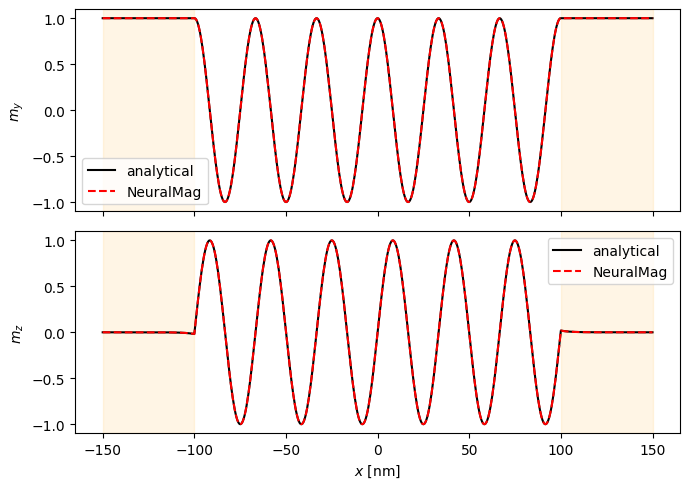
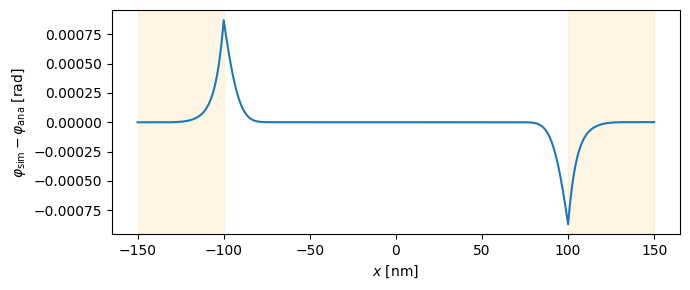
The shaded regions indicate the ferromagnetic slabs. The simulated magnetisation matches the analytical helix to within the discretisation error of the nodal finite-difference method. For a quantitative assessment one can compute the phase \(\varphi\) from the components and plot its deviation from the analytical profile.
[10]:
phi_sim = np.unwrap(np.arctan2(m_np[:, 2], m_np[:, 1]))
phi_ref_u = np.unwrap(phi_ref)
phi_sim += phi_ref_u[(N + 1) // 2] - phi_sim[(N + 1) // 2]

plt.figure(figsize=(7, 3))
plt.plot(x_n * 1e9, phi_sim - phi_ref_u)
plt.axvspan(-L * 1e9, -L0 * 1e9, color="orange", alpha=0.1)
plt.axvspan(L0 * 1e9, L * 1e9, color="orange", alpha=0.1)
plt.xlabel(r"$x$ [nm]")
plt.ylabel(r"$\varphi_{\mathrm{sim}} - \varphi_{\mathrm{ana}}$ [rad]")
plt.tight_layout()
plt.show()