Time dependent optimization (JAX version)

In this example, we use the inverse computing capibilities of NeuralMag in order to optimize the direction of an external field in order to control the magnetization dynamics of a single-domain particle. Specifilly, the field is optimized such that the magnetization is pointing in a given direction \(\vec{m}_\text{target}\) at time \(T\). This example is taken from [1] and reads

\[\begin{split}\begin{align} \vec{H}_\text{ext}(\theta, \phi) &= H_c \begin{pmatrix} \sin(\theta) \cos(\phi)\\ \sin(\theta) \sin(\phi)\\ \cos(\theta) \end{pmatrix},\\ \vec{H}_\text{eff} &= \vec{H}_\text{aniso} + \vec{H}_\text{exchange} + \vec{H}_\text{ext},\\ \mathcal{L}(\theta, \phi) &= \int_{\Omega} \|\vec{m}(T) - \vec{m}_\text{target}\| \,\text{d}V. \end{align}\end{split}\]

Simulation

For this example, we use the JAX backend together with the Optax library for optimiz ### Import libraries Import libraries, set backend to JAX and reduce FEM quadrature order for better performance.

import equinox as eqx
import jax.numpy as jnp
import matplotlib.pyplot as plt
import numpy as np
import optax
from scipy import constants
from tqdm import tqdm

import neuralmag as nm

nm.config.backend = "jax"
nm.config.fem["n_gauss"] = 1

2025-05-13 11:23:09 NeuralMag:INFO [NeuralMag] Version 0.9.1
2025-05-13 11:23:09 NeuralMag:INFO [NeuralMag] Backend set to 'jax'.

Setup mesh and state

Setup mesh, state and material parameters and set initial magnetization in z-direction.

mesh = nm.Mesh((2, 2, 2), (5e-9, 5e-9, 5e-9))
state = nm.State(mesh)

state.material.Ms = 8e5
state.material.A = 1.3e-11
state.material.Ku = 1e5
state.material.Ku_axis = [0, 0, 1]
state.material.alpha = 0.1

state.m = nm.VectorFunction(state).fill((0, 0, 1))

2025-05-13 11:23:09 NeuralMag:INFO [Mesh] 3D, 2 x 2 x 2 (size = 5e-09 x 5e-09 x 5e-09)
2025-05-13 11:23:09 NeuralMag:INFO [NeuralMag] Set default device to 'TFRT_CPU_0'.
2025-05-13 11:23:09 NeuralMag:INFO [NeuralMag] Set default dtype to 'float32'.
2025-05-13 11:23:09 NeuralMag:INFO [State] Running on device: TFRT_CPU_0 (dtype = float32, backend = jax)

Set up external-field function

Next, we set up the external-field function as dynamic attribute depending and the spherical angles \(\phi\) and \(\theta\).

H = 2 * 1e5 / (constants.mu_0 * 8e5)
state.phi = lambda angles: angles[0]
state.theta = lambda angles: angles[1]
state.angles = [jnp.pi / 2, jnp.pi / 2]
h_ext = lambda angles: jnp.stack(
    [
        H / 2 * jnp.sin(angles[0]) * jnp.cos(angles[1]),
        H / 2 * jnp.sin(angles[0]) * jnp.sin(angles[1]),
        H / 2 * jnp.cos(angles[0]),
    ]
)

Set up effective field

nm.ExchangeField().register(state, "exchange")
nm.UniaxialAnisotropyField().register(state, "aniso")
nm.ExternalField(h_ext).register(state, "external")
nm.TotalField("exchange", "aniso", "external").register(state)

2025-05-13 11:23:09 NeuralMag:INFO [ExchangeField] Register state methods (field: 'h_exchange', energy: 'E_exchange')
2025-05-13 11:23:09 NeuralMag:INFO [UniaxialAnisotropyField] Register state methods (field: 'h_aniso', energy: 'E_aniso')
2025-05-13 11:23:09 NeuralMag:INFO [ExternalField] Register state methods (field: 'h_external', energy: 'E_external')
2025-05-13 11:23:09 NeuralMag:INFO [TotalField] Register state methods (field: 'h', energy: 'E')

Set up LLGSolver

Next, we set up the LLGSolver defining angles as parameters in order to allow for efficient gradient computation.

llg = nm.LLGSolver(state, parameters=["angles"])

2025-05-13 11:23:09 NeuralMag:INFO [LLGSolverJAX] Initialize RHS function

Define loss function

We define the target magnetzation m_target and the loss function grad_loss. Note the use of the filter_value_and_grad decorator that enriches the return value of the loss with its gradient.

m_target = nm.VectorFunction(state).fill((0.5**0.5, 0, 0.5**0.5)).tensor


@eqx.filter_value_and_grad
def grad_loss(angles):
    m_pred = llg.solve(state.tensor([0.0, 0.05e-9]), angles).ys[-1]
    return jnp.mean((m_target - m_pred) ** 2)

Set up optimizer

Now, we define a step function for the optimization and set up an AdaBelief optimizer with a learning rate of 0.05.

@eqx.filter_jit
def make_step(angles, opt_state):
    loss, grads = grad_loss(angles)
    updates, opt_state = optim.update(grads, opt_state)
    angles = eqx.apply_updates(angles, updates)
    return loss, angles, opt_state


optim = optax.adabelief(0.05)
opt_state = optim.init(state.angles)

Perform optimization loop

logger = nm.ScalarLogger("time-dependent-optimization_jax/log.dat", ["step", "phi", "theta", "loss"])
for step in tqdm(range(100)):
    state.step = step
    state.loss, state.angles, opt_state = make_step(state.angles, opt_state)
    logger.log(state)

100%|█████████████████████████████████████████████████████████████████████████████████████████████████████████████████████████████████████████████████████████████████████████████| 100/100 [00:49<00:00,  2.01it/s]

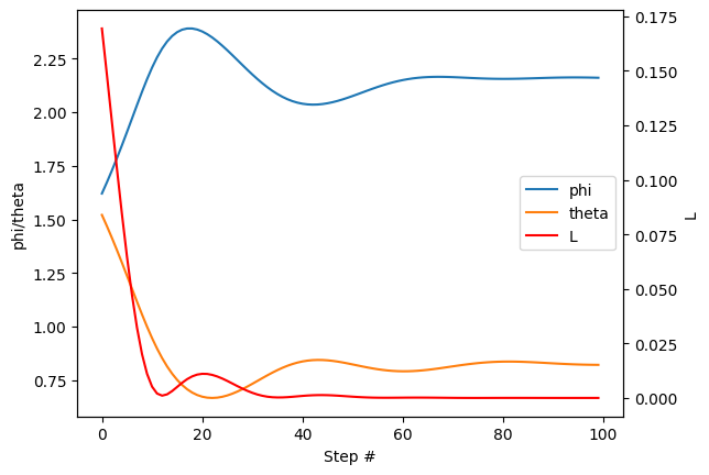
Plot the solution

Finally, we plot the evolution of the field angles along with the loss function against the number of optimization steps.

data = np.loadtxt("time-dependent-optimization_jax/log.dat")
fig, ax1 = plt.subplots()
(l1,) = ax1.plot(data[:, 0], data[:, 1], label="phi")
(l2,) = ax1.plot(data[:, 0], data[:, 2], label="theta")
ax1.set_xlabel("Step #")
ax1.set_ylabel("phi/theta")

ax2 = ax1.twinx()
(l3,) = ax2.plot(data[:, 0], data[:, 3], label="L", color="red")
ax2.set_ylabel("L")

lines = [l1, l2, l3]
labels = [line.get_label() for line in lines]
ax1.legend(lines, labels, loc="best")

plt.show()