Shape optimization with a level-set parameterization (JAX version)

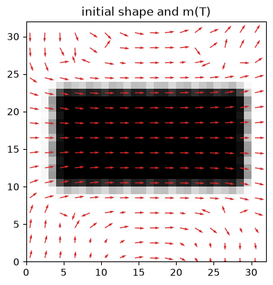
In this example we use the LevelSetParameterization class to perform a free-form shape optimization in which the demag field is the only actuator. A soft-magnetic 2D element starts as a rectangle elongated along \(x\) with uniform magnetization \(\vec{m} = \vec{e}_x\) – its shape-anisotropy easy axis, i.e. an equilibrium. The RBF amplitudes of the level-set parameterization (the element’s shape) are optimized such that the magnetization, relaxing for \(T = 2\,\text{ns}\) under exchange and demag interaction only, ends up along \(+y\):

\[\mathcal{L}(\vec{s}) = \frac{\int_\Omega \rho(\vec{s}) \, \|\vec{m}(T) - \vec{m}_\text{target}\|^2 \,\text{d}V}{\int_\Omega \rho(\vec{s}) \,\text{d}V}, \qquad \vec{m}_\text{target} = \vec{e}_y.\]

Since the easy axis follows the shape, the optimizer has to rotate the element’s elongation from \(x\) to \(y\). The level-set parameterization is free to change the topology of the design along the way – nucleating holes or splitting the element into several islands – which distinguishes it from boundary-based shape optimization.

Import libraries

Import libraries and set the backend to JAX. The level-set smooth maximum requires float64: under float32 it loses accuracy, and reverse-mode gradients through the LLG time integration have been observed to be NaN while the forward pass looks healthy. The dtype must be set before any tensor is created.

import equinox as eqx
import matplotlib.pyplot as plt
import numpy as np
import optax
from tqdm import tqdm

import neuralmag as nm

nm.config.backend = "jax"
nm.config.dtype = "float64"

/home/av09084/envs/neuralmag_nodefix/lib/python3.13/site-packages/tqdm/auto.py:21: TqdmWarning: IProgress not found. Please update jupyter and ipywidgets. See https://ipywidgets.readthedocs.io/en/stable/user_install.html
  from .autonotebook import tqdm as notebook_tqdm
2026-09-03 15:09:18 NeuralMag:INFO [NeuralMag] Version 1.0.0
2026-09-03 15:09:19 NeuralMag:INFO [NeuralMag] Backend set to 'jax'.
2026-09-03 15:09:19 NeuralMag:INFO [NeuralMag] Set default dtype to 'float64'.

Setup mesh and state

Setup mesh, state and material parameters. The damping is set to \(\alpha = 1\): only the final state matters in this example, not the dynamics of \(\vec{m}\), so the strongly overdamped \(\vec{m}(T)\) approximates the equilibrium of the current shape rather than a mid-precession snapshot.

mesh = nm.Mesh((32, 32), (5e-9, 5e-9, 5e-9))
state = nm.State(mesh)

state.material.Ms = 8e5
state.material.A = 1.3e-11
state.material.alpha = 1.0

2026-09-03 15:09:19 NeuralMag:INFO [Mesh] 2D, 32 x 32 (size = 5e-09 x 5e-09 x 5e-09)
2026-09-03 15:09:20 NeuralMag:INFO [NeuralMag] Set default device to 'cpu:0'.
2026-09-03 15:09:20 NeuralMag:INFO [State] Running on device: cpu:0 (dtype = float64, backend = jax)

Set up the level-set parameterization

The design region covers the mesh up to a 2-cell border. Note that outside the design region the parameterization places material (\(\rho = 1\)), so that a design can be embedded in a fixed layout; here the geometry mask turns that border into permanent void instead, keeping the element away from the mesh edge.

The initial shape is a rectangle elongated along \(x\) (half-widths 12 x 6 cells): positive amplitudes inside, negative outside put the level-set interface at the rectangle’s edge. The interface must lie inside the mesh – if the sigmoid saturates everywhere (no interface), the gradient with respect to the amplitudes is exactly zero and the optimization cannot start.

sigmoid_a sets the interface width: with the default Eikonal renormalization the 10–90 % transition of \(\rho\) spans about \(4/a\) cells, so sigmoid_a=3 gives an interface about 1.3 cells wide, independently of the design and of the filter width.

NUM_RBFS = 10
BORDER = 2

geometry = np.ones(mesh.n)
geometry[:BORDER, :] = geometry[-BORDER:, :] = 0.0
geometry[:, :BORDER] = geometry[:, -BORDER:] = 0.0

lsf = nm.LevelSetParameterization(
    NUM_RBFS,
    NUM_RBFS,
    xlimits=(BORDER, mesh.n[0] - BORDER),
    ylimits=(BORDER, mesh.n[1] - BORDER),
    geometry=geometry,
    sigmoid_a=3.0,
)
lsf.register(state)

centers_x = np.linspace(BORDER, mesh.n[0] - BORDER, NUM_RBFS)
centers_y = np.linspace(BORDER, mesh.n[1] - BORDER, NUM_RBFS)
cx, cy = np.meshgrid(centers_x, centers_y, indexing="ij")
inside = (np.abs(cx - mesh.n[0] / 2) < 12.0) & (np.abs(cy - mesh.n[1] / 2) < 6.0)
state.rbf_amplitudes = state.tensor(np.where(inside, 2.0, -2.0))

rho_func = state.resolve("rho", ["rbf_amplitudes"])

2026-09-03 15:09:20 NeuralMag:INFO [LevelSetParameterization] Register state method 'rho' (10x10 RBFs on cells x(2, 30), y(2, 30))

Set up magnetization and effective field

The magnetization starts uniformly along \(+x\), the easy axis of the initial rectangle. The torque on this initial configuration is close to zero – but the gradient with respect to the amplitudes is not, since asymmetric shape changes tilt the demag field. The magnetization is defined as a cell function on the same grid as \(\rho\), so the loss needs no interpolation between nodes and cells. The effective field consists of exchange and demag interaction only – there is no external field in this example.

state.m = nm.VectorCellFunction(state).fill((1.0, 0.0, 0.0))

nm.ExchangeField().register(state, "exchange")
nm.DemagField().register(state, "demag")
nm.TotalField("exchange", "demag").register(state)

2026-09-03 15:09:20 NeuralMag:INFO [ExchangeField] Register state methods (field: 'h_exchange', energy: 'E_exchange', energy density: 'e_exchange')
2026-09-03 15:09:20 NeuralMag:INFO [DemagField] Register state methods (field: 'h_demag', energy: 'E_demag', energy density: 'e_demag')
2026-09-03 15:09:20 NeuralMag:INFO [DemagField]: building the demag tensor on the CPU (NumPy). Set NM_JAX_GPU_SETUP=1 or pass gpu_setup=True (requires PyTorch and a CUDA GPU) to build it on the GPU -- much faster for large meshes.
2026-09-03 15:09:20 NeuralMag:INFO [DemagField]: Set up demag tensor
2026-09-03 15:09:21 NeuralMag:INFO [TotalField] Register state methods (field: 'h', energy: 'E', energy density: 'e')

Set up LLGSolver

The RBF amplitudes are registered as solver parameters in order to allow for efficient adjoint gradient computation through the time integration.

llg = nm.LLGSolver(state, parameters=["rbf_amplitudes"])

ts = state.tensor([0.0, 2e-9])
m_target = state.tensor([0.0, 1.0, 0.0])

2026-09-03 15:09:21 NeuralMag:INFO [LLGSolverJAX] Initialize RHS function

Define loss function

The loss is the \(\rho\)-weighted misalignment between \(\vec{m}(T)\) and the target direction. The weighting keeps the void region – where the magnetization is physically meaningless – out of the loss, and the normalization avoids rewarding plain material removal. The filter_value_and_grad decorator enriches the return value of the loss with its gradient.

@eqx.filter_value_and_grad
def grad_loss(amps):
    m_T = llg.solve(ts, amps).ys[-1]
    rho = rho_func(amps)
    return (rho * ((m_T - m_target) ** 2).sum(-1)).sum() / rho.sum()

Define plot function

Visualize a design \(\rho\) together with the relaxed magnetization \(\vec{m}(T)\) on it.

def plot_design(amps, title):
    m_T = np.asarray(llg.solve(ts, amps).ys[-1])
    rho = np.asarray(rho_func(amps))
    fig, ax = plt.subplots(figsize=(4.5, 4.5))
    ax.imshow(rho.T, origin="lower", cmap="gray_r", vmin=0, vmax=1, extent=(0, mesh.n[0], 0, mesh.n[1]))
    sl = slice(None, None, 2)
    X, Y = np.meshgrid((np.arange(mesh.n[0]) + 0.5)[sl], (np.arange(mesh.n[1]) + 0.5)[sl], indexing="ij")
    ax.quiver(X, Y, m_T[sl, sl, 0], m_T[sl, sl, 1], color="tab:red", scale=25)
    ax.set_title(title)
    plt.show()


plot_design(state.rbf_amplitudes, "initial shape and m(T)")

Verify gradient flow

Before optimizing, check that the gradient through the time integration is finite and non-zero. If this assert fires, the initial design has no interface inside the mesh (see above) or the state is not float64.

loss, grad = grad_loss(state.rbf_amplitudes)
assert np.all(np.isfinite(grad)) and np.abs(grad).max() > 0.0
print(f"initial loss = {float(loss):.4f}, max |dL/ds| = {np.abs(np.asarray(grad)).max():.2e}")

initial loss = 1.9999, max |dL/ds| = 2.68e-01

Set up optimizer

We use the AdaBelief optimizer with a learning rate of 0.01. The small learning rate matters here: adaptive optimizers keep moving the design at roughly the learning rate even after convergence, and larger rates can drift the converged design onto configurations where the relaxed magnetization flips between the degenerate \(\pm y\) equilibria, which shows up as spikes in the loss curve.

optim = optax.adabelief(0.01)
opt_state = optim.init(state.rbf_amplitudes)


@eqx.filter_jit
def make_step(amps, opt_state):
    loss, grads = grad_loss(amps)
    updates, opt_state = optim.update(grads, opt_state)
    amps = eqx.apply_updates(amps, updates)
    return loss, amps, opt_state

Perform optimization loop

amps = state.rbf_amplitudes
history = []
for step in tqdm(range(200)):
    loss, amps, opt_state = make_step(amps, opt_state)
    history.append(float(loss))

state.rbf_amplitudes = amps

100%|██████████| 200/200 [03:47<00:00,  1.14s/it]

Plot the solution

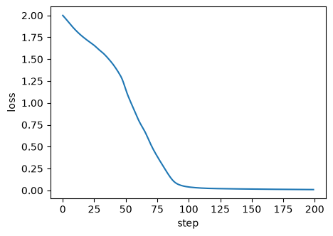
The loss decreases smoothly; the shoulder around step 70 marks the transition of the design between shape configurations. Note that the loss measures a dynamical snapshot at \(t = T\), and near configurations where the relaxation slows down it is a very sensitive function of the shape.

plt.figure(figsize=(5, 3.5))
plt.plot(history)
plt.xlabel("step")
plt.ylabel("loss")
plt.show()

print(f"final loss = {history[-1]:.4f}")

final loss = 0.0094

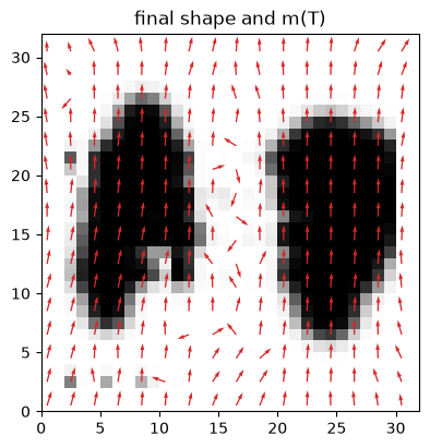
The optimized design splits the initial rectangle into two islands elongated along \(y\) – a topology change that a boundary-based shape optimization could not perform – and the magnetization, driven by shape anisotropy alone, follows their long axis into the target direction.

plot_design(amps, "final shape and m(T)")

m_T = np.asarray(llg.solve(ts, amps).ys[-1])
rho = np.asarray(rho_func(amps))
m_mean = (rho[..., None] * m_T).sum((0, 1)) / rho.sum()
print(f"rho-weighted <m>(T) = ({m_mean[0]:+.3f}, {m_mean[1]:+.3f}, {m_mean[2]:+.3f})")

rho-weighted <m>(T) = (+0.069, +0.995, -0.000)